Generating Schedules
At the core of Non Uniform Sampling and reconstructing of the resultant spectra is selecting which points to acquire and which to skip. Work in our lab has established the Poisson Gap Sampling Method (Hyberts et al, JACS, 2010) results in superior schedules with fewer artifacts during Forward Maximum Entropy reconstruction. Empirical evidence from our lab (unpublished) suggests this is also true for the Iterative Soft Threshold algorithm. You can create your own schedules using our Poisson Gap Schedule Java applet. Download it here.
Launching the Java Applet
On unix and MacOSX systems, from the command line type:
- java -jar PoissonGap2.jar
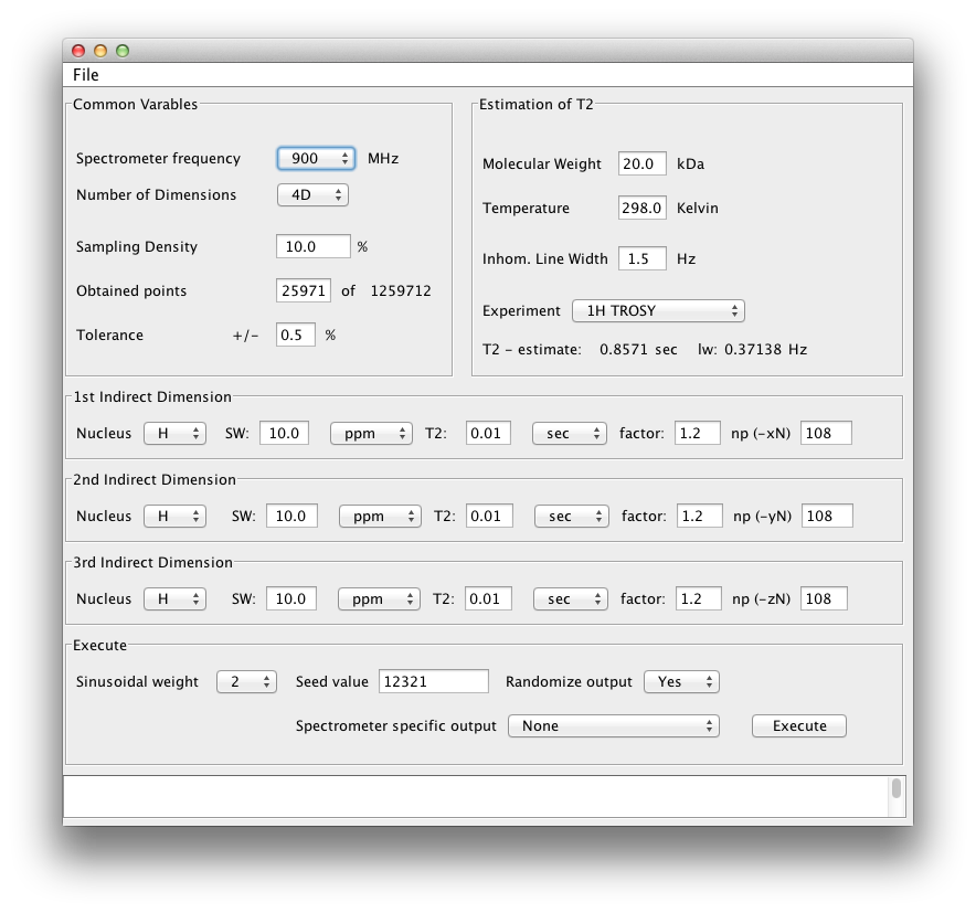
You will be greeted with the following window with defaults set up for collecitng a 4D spectrum.
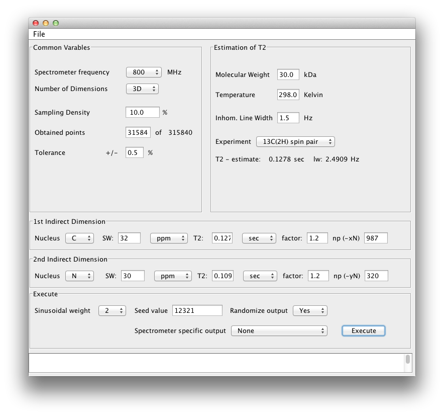
Our 3D example is for a triple resonance TROSY HNCA spectrum collected on a 30 kDa protein at 800 MHz. The scheduler should be set up as below:
Lets go over the details.
Setting up the Scheduler
The top left box is titled "Common Variables". Here we set the spectrometer frequency and number of dimensions. 3D means there are three dimensions collected, including the direct dimension, i.e. 3D = 1 direct and 2 indirect (non uniformly sampled) dimensions. We will return to the rest of the variables here in a moment.
Setting up T2 estimates for indirect dimensions.
The top right box is used to estimate the rate of relaxation of the signal in a particular dimension. This is estimated fom the molecular weight, temperature and the experiment type (or nature of the transverse magnetization in a particular dimension). We also include field inhomogeneity (typically 1.5 Hz but sometimes you can shim better than this). The experiment type has a few options. See below:
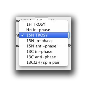
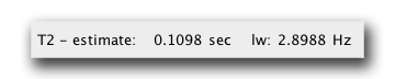
Select the most appropriate one. For example, our TROSY HNCA will use 15N TROSY in the N dimension. This will yield a T2 relaxation time of 0.1098 seconds.
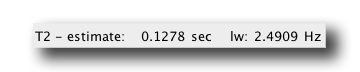
Our trosy HNCA is most likely on a deuterated protein, so to estimate the T2 relaxation time of the CA nucleus, we use the 13C(2H) spin pair. This yields a T2 relaxation time of 0.1278 seconds.
We now insert these T2 numbers into the areas labeled 1st Indirect Dimension and 2nd Indirect Dimension. By convention, our triple resonance non uniform sequences will always have the 1st indirect dimension as the carbon dimension and the 2nd indirect dimension will be the nitrogen dimension. This also translates into the carbon dimension being the slowly acquired dimension while the Nitrogen dimension is 'fast' acquired. First, put in the sweep width for each dimension. Below we have entered a SW of 32 ppm for the CA (typical) and a SW of 30 for N (typical). The figure below also shows these boxes with the T2 times determined above placed in the T2 box. If you press enter in this box, the app automatically determine the optimum number of points to acquire for maximum signal to noise given the T2 times estimated above (see Rovnyak 2004.)
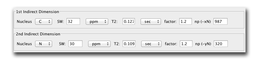
We see maximum signal to noise is acquired in the CA dimension after 987 points! If only this was actually doable! In the N dimension we see 320 points is optimal.
Technical Considerations for Number of Points Collected
Now with an indirect matrix of 987 by 320 points, this totals to 315840 points to acquire indirectly. This is impractical. Now, non uniform sampling permits sampling a subset of these points. However, even sampling 1% of these points results in >3000 points. This could be collected in a reasonable time, however we have seen empirically that colecting 1% of points in 3D experiments can lead to reconstruction artifacts.
Scott's Rule of Thumb:The minimum percentage of points to acquire in a 3D experiment is ~5-10%. In 4D experiments, you should collect more than 0.5%. These are only guidlines based on our experience. We are working on establishing more rigid guidlines.
In this trosy HNCA example we wish to collect 10% of points. One of the first considerations is are any of the dimensions acquired in 'constant time', e.g. the N dimension. If so, the number of points that can be acquired is limited. Typically a constant time N dimension at 800 MHz will only permit the acquisition of ~64 points (and even less if using concatenated sequences). Setting the N dimension points to 64 results in a matrix of 987 * 64 = 63168 points. 10% of these is now only ~6000 points.
The scheduler will now look like this:
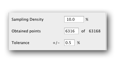
And there will be 63168 points to acquire, 10% of which is ~6300. This is still a lot of points. To cut down on points you can cut the numbers of points in the C dimension. How much you cut it depends on how many points you can afford to collect in how much time. We find that acquiring 128 points in C along with 64 points in N and then subsampling 10% has always worked for us. This means collecting only ~820 points. Obviously 128 indirect carbon points is much shorter than the expected maximum of >900 points, but we find we can artifically extend this dimension during reconstruction. More details on that in the reconstruction part.
Outputting a Schedule
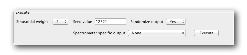
There are three variables to set before outputting a schedule. The sinusoidal weight (0, 1 or 2), a random seed (a random integer) and an option to randomize the order of the output schedule (yes or no). There is also spectrometer sepcific output options, but we wont discuss these for now. Play with them yourself.
Sinusiodal Weight
Sinusiodal weight refers to the way the points are weighted in the schedule. A value of 0 means they are not weighted at all and will be evenly distributed. A sinusoidal weight of 2 means the gap probability at a point along the schedule is proprtional to sin(0) to sin(pi/2) along the schedule. For a sin weighting of 1 the probabilty is proportional to sin(0) to sin(pi/1). For more details, see Hyberts, 2009.
Seed Value
This is just a random number to start the random number generator for the scheduler. Use any number you want here or take the default
Randomize Output
The schedule can be outputted in a random order so points are not acquired with ever increasing delay times. This may be a fairer way of collecting points, however when learning this procedure it is best to stick with an ordered output so set it to 'no'. Having an ordered output helps in determining if you are acquiring your spectrum correctly when sittng at the console.
Output time!
Now just press Execute and follow the dialogs. An example output text file looks like this:
0 0 0 1 0 2 0 3 0 4 0 5 0 6 0 7 0 9 0 11 0 13 0 16 0 17 0 21 0 23 0 27 0 32 0 40 0 48 0 59 . . . . . . 127 17 127 35 127 50
From this you can see the first column is the slow dimension (C) and the second column is a the fast dimension (N). It is important to understand the order because the order of the schedule much match the order the pulse sequence expects. For example, most of our pulse sequences will use the second column first and the first column second. We will provide scripts that convert these sequences to the appropriate format for our pulse sequences.
Now you are ready to move on to setting up the experiment with your schedule. Go to the next tab!